Information Theory Assignment
First, a couple of notes.
For the mathematically inclined and/or those who liked the idea of
deriving an information measure from a set of properties such a measure should have,
here are several derivations
of the definition of entropy based on axioms about such
properties.
The one I mentioned in class is from A.I. Khinchin,
Mathematical Foundations of Information Theory, Dover, New
York, 1957.
Also, in case you're curious, here's the pointer to an algorithm for
creating optimal codes using Huffman coding
(see also this interesting
discussion by Huffman's nephew).
Finally, a reminder about notation. If X is a random variable whose distribution
is (p1,p2,...,pk) then we usually
write H(X) for H(p1,p2,...,pk). I will
occasionally write H(p) instead of H(X), where p abbreviates
p1,p2,...,pk.
Do BOTH of these on-paper problems
-
(Manning and Schuetze exercise 2.12) Show that the KL divergence
is not symmetric by giving an example of two distributions p and q
for which D(p||q) is not equal to D(q||p). Give the two distributions
and show the explicit computation of the KL divergences.
Note that if you understand KL-divergence, this problem should take you no more than 5 minutes, including writing it down. If it's taking you longer, go back and make sure you understand what KL-divergence is.
Also note that simple toy distributions (e.g. over {heads,tails}) are really boring to grade! You can give us the boring kind of example, but you'll earn more goodwill for an example that is significantly interesting or amusing.
-
- a. Consider a set of eight horses, h0-h7, that repeatedly race
each other. Suppose the probability distribution over horses h0-h7
for winning a race is p:
	       h0     h1   h2     h3     h4     h5     h6     h7
	 p     1/2    1/4  1/8    1/16   1/64   1/64   1/64   1/64
For any probability distribution, an optimal binary
representation of the events, in the sense of requiring the smallest number of bits
on average to communicate outcomes, can be created using Huffman
coding. Here's the encoding you'd get for the above distribution:
	       h0     h1   h2     h3     h4     h5     h6     h7
      codeP    0      10   110    1110   111100 111101 111110 111111
Illustrate using codeP that the expected value of the length Ep[length(h)] is equal to H(p), the
entropy of the distribution. You can simply do the two
computations numerically using codeP and confirm that you get the same number,
though you'll understand what's going on better if you look at the definitions
of Ep[length(h)] and H(p) and show that one is equivalent to the other.
-
b. Imagine that p is the true distribution of outcomes when these
horses race, but that we do a terrible job of estimating the probabilities
and come up with the following model, q:
	       h0     h1   h2     h3     h4     h5     h6     h7
	 q     1/8    1/8  1/8    1/8    1/8    1/8    1/8    1/8
Since the horses all have the same probability, there's no basis
for distinguishing them, so obviously the best code we
can invent will use the same number of bits for each
horse. This means that the smallest number of bits we can use is
log28 = 3 bits:
	       h0     h1   h2     h3     h4     h5     h6     h7
      codeQ   000    001  010    011    100    101    110    111
Now imagine that we communicate lots of horse race outcomes using
codeQ. Encoding winning horses using codeQ, what is
Ep[length(h)]?
- c. Use the previous two parts to this question, together with the definition
of relative entropy (KL divergence), to explain and illustrate
Manning and Schuetze's observation: "KL divergence is the
average number of bits that are wasted by encoding events from
a distribution p with a code based on a not-quite-right
distribution q."
Do ONE of the following TWO exercises in programming and data exploration
Option 3a
Read Piantadosi et al. (2011), Word lengths are optimized for efficient communication, showing that word length correlates better with the average amount of information conveyed by a word in context than it does with the word's context-independent frequency or information. (Wait, you mean you didn't already read it for last class?!)
This seems like it should be a really easy do-it-yourself experiment -- so the problem is to have a try at doing it yourself!
You can do this for the simple case of just bigram probabilities (i.e. context C=c means "the previous word is c"), although it would certainly also be interesting to see what things look like for higher-order ngrams. If you're doing that, I recommend using an existing language modeling module (e.g. in NLTK) or toolkit (e.g. KenLM and SRILM). As usual, just make sure to clearly identify any software that you didn't write yourself in your PDF writeup.
You should do your experiment for English and at least one other language.
As one possible source of data to work with, see the NLTK corpora. The Brown corpus would be a smallish but decent source for English (just remove POS tags and lowercase everything; it's already tokenized); you could also augment that with other English corpora, although be careful to make sure that your sources don't overlap, which would throw off your counts. For other languages, one source would be the NLTK samples from the Europarl corpora; if you were feeling more ambitious you could look into the full Europarl corpora, which I believe are quite a bit larger. Or feel free to identify other sources of text. The corpus processing (acquisition, cleanup, etc.) are not the point of this assignment, so I encourage people to share pointers, cleanup code, and even corpus data using Piazza. (Recall that constructive participation on Piazza contributes to your class participation grade.)
You are not required to actually succeed in replicating the research results in the paper -- that would take a lot of work, since they used fairly sizeable corpora that you probably don't have easy access to. In fact, you're not even required to compute correlations (though that would be nice); we'll be happy if you produce charts that look roughly like their Figure 2, no error bars required (though that would be nice also).
What you do need to do involves (a) briefly summarizing what the study is about in your own words to show that you understand it, (b) clearly describing for us what you did in your own experiment (along with any simplifying choices you made and why/how you made them), and (c) clearly showing and telling us what you you found. If your results are very different from what you would have expected, then (d) suggest some explanations why (and ideally support your explanation with data). The more thoughtful and clearly written your writeup the better.
Remember that the goal is not to "get it right", but to show you understand the ideas and that you're taking a thoughtful approach. The writeup matters.
By the way, if you found this interesting, there's a follow-up paper in which Meylan and Griffiths (2017) argue that phonological distinctiveness actually outperforms word length as a predictor of frequency. They define the phonological information content of a word to measure
the distinctiveness of its phoneme-to-phoneme transitions. The intuition behind their argument is that it's not just a word's probability in context that influences how much effort it takes to recognize it -- it's also the number of competitors (alternative words) you could have been hearing at that point based on the acoustic evidence.
Option 3b
(Based very loosely on Manning and Schuetze exercise 2.10) For this problem, let's use the State of the Union(SOTU) addresses of U.S. presidents, a collection of documents described in the previous assignment. For our purposes here, let's restrict ourselves to Presidents Bush-1 (that is, Republican president George Herbert Walker Bush), Clinton (Democrat), Bush-2 (that is, Republican president George W. Bush), and Obama (Democrat). For simplicity, you can assume that the total vocabulary is the union of all the unigrams in the various texts.
To answer the questions you'll need to estimate probability distributions over unigrams for each president.
Speeches will of course need to be tokenized, and you should
convert all text to lowercase in order to mitigate sparse data problems. Note that you'll need to do something about zero
counts. As the simplest option, you can smooth using Laplace smoothing ("add
one", Manning and Schuetze Section 6.2.2) to avoid zero, even though
in practice this is not considered the state of the art. (Ok, I'm probably being overly generous. In these tutorial slides about smoothing the author describes Laplace as "a horrible choice".) Or, a bit better, you could use add-k for a different k, e.g. setting k to 1/|V| where |V| is the size of the vocabulary. That's really easy to implement, if you're programming from scratch, and it tends to work ok. State of the art would be modified Kneser-Ney smoothing, though it would be a major distraction from the main point of the assignment for you to implement that from scratch.
Here's a simple observation that might help you avoid writing a lot of
new code from scratch, allowing you to re-use work you've already done
in the previous assignment: if you have a bigram frequency table with
entries count(a,b), then the unigram counts are just the marginal
counts for a and b, i.e.:
count(a) = ∑b' count(a,b')
count(b) = ∑a' count(a',b)
Best practice would be to smooth the bigram counts first, and then
compute the unigram counts as above. If you smooth unigrams and
bigrams separately, there's no guarantee that summing over smoothed
bigram counts to compute the marginals will give you the same number
you get from smoothing unigrams separately. But this is a minor point
and for this assignment I'm fine with any fairly reasonable smoothing
as long as you say clearly what you did.
Speaking of implementing from scratch, you don't have to do everything completely from scratch. There are, for example, existing language modeling modules (e.g. in NLTK) and toolkits (e.g. KenLM and SRILM), and these days it's also not difficult to find code for neural network language models, e.g. OxLM or this tutorial on implementing a recurrent neural network language model using Theano; see also the CL1 notes on
n-gram language models and
neural language models.
You're welcome to use tools like those in any way you like -- just make sure to clearly identify any software that you didn't write yourself in your PDF writeup. And if you find a particularly good discussion/tutorial on the Web, please post it to the class discussion board!
Questions.
- a. Treating the distribution for the Obama speeches as p, the Bush-2 speeches as q, and the Clinton speeches as q', what are D(p||q) and D(p||q')? How well does this match what you expected them to be? Explain your answer.
- b. What are the top 10 terms contributing to the KL divergence in both cases? Suggest reasons these might be the top 10. (If you don't find anything interesting in the top 10, you're welcome to look at more.)
- c. Build two unigram language models using the Bush-1 speeches and the Clinton speeches, and evaluate those two models using the Bush-2 speeches as the language L that represents "truth". What is the perplexity of each model, and which of the two is a better model for Bush-2's speeches? Does this fit with what you would have expected? Why or why not?
Extra credit (up to 10%)
The idea for this extra credit is to do an analysis similar in spirit to the Civis Analytics blog posting, but exercising things you've learned in class. As long as you meet that goal, if you want to do something a little different from exactly what I'm suggesting here, because of your own interests, that's fine -- make it interesting!
- For all the individual SOTU speeches from Bush-2 to the present (inclusive), build a similarity matrix like the one in the Civis Analytics blog posting, e.g. here is the fragment for the Obama speeches:
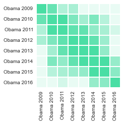 .
As your measure comparing any two speeches, use (1/2)*(D(p||q)+D(q||p)), where p and q are bigram distributions for the two speeches being compared. (Averaging the two KL-diverence values is a common way of producing a symmetric value. For related discussion see the Wikipedia page on Jensen-Shannon divergence.)
The result can be just a big table of numbers, if you like, though if you want to do a nice-looking matrix heatmap there are many packages for that, e.g. see this one.
a. Show the table that you constructed (or the heatmap).
b. Does the matrix look like you would have expected? Are there any surprises, and if so, what's your explanation? (If you want to explore what's going on in a data-driven way, you could take inspiration from question 3b, above.)
c. How do your table and analysis compare with what's in the Civis Analytics posting? Is what you're seeing generally similar? Any interesting differences? Again, do you have any thoughts about why you might or might not be seeing differences?